Getting started

CausalDynamics supplies graphs, d-separation, and identification certificates for structural and discrete-time models. The walk-throughs below run in Documenter with small examples you can copy into scripts or Quarto chunks.

Install from General:

using Pkg
Pkg.add("CausalDynamics")

Load DAGMakie when you want figures (using DAGMakie, CairoMakie activates the plotting extension):

using CausalDynamics, Graphs, DAGMakie, CairoMakie

DAG figures follow Cinelli, Forney & Pearl (2022, SMR): a good-control triangle for adjustment, then the estimand path with effects on edges where helpful. Plotting uses DAGMakie directly (dagplot_confounding, dagplot_backdoor, dagplot_chain, dagplot_mediation, dagplot_temporal, edge_routing, CurvedEdge).

1. Backdoor adjustment (good control)

Graph. Classic confounding: Z → X → Y and Z → Y.

using CausalDynamics, Graphs

g = DiGraph(3)
add_edge!(g, 1, 2)  # Z → X
add_edge!(g, 1, 3)  # Z → Y
add_edge!(g, 2, 3)  # X → Y
names = Dict(1 => :Z, 2 => :X, 3 => :Y)

d_separated(g, 2, 3, [1])  # false: direct X → Y path remains open
backdoor_adjustment_set(g, 2, 3)  # Set([1])

Set{Int64} with 1 element:
  1

Conditioning on Z blocks the backdoor path X ← Z → Y, but not the direct causal path X → Y. Thus, Z satisfies the backdoor criterion while X and Y remain d-connected given Z.

Graph (identification). Good-control triangle: adjust Z (Cinelli et al. 2022).

using DAGMakie, CairoMakie

fig, _, _ = dagplot_confounding(["Z", "X", "Y"];
    color_by = :adjustment,
    exposure = 2,
    outcome = 3,
    adjustment = Set([1]),
    title = "Good control Z (identification)",
)
fig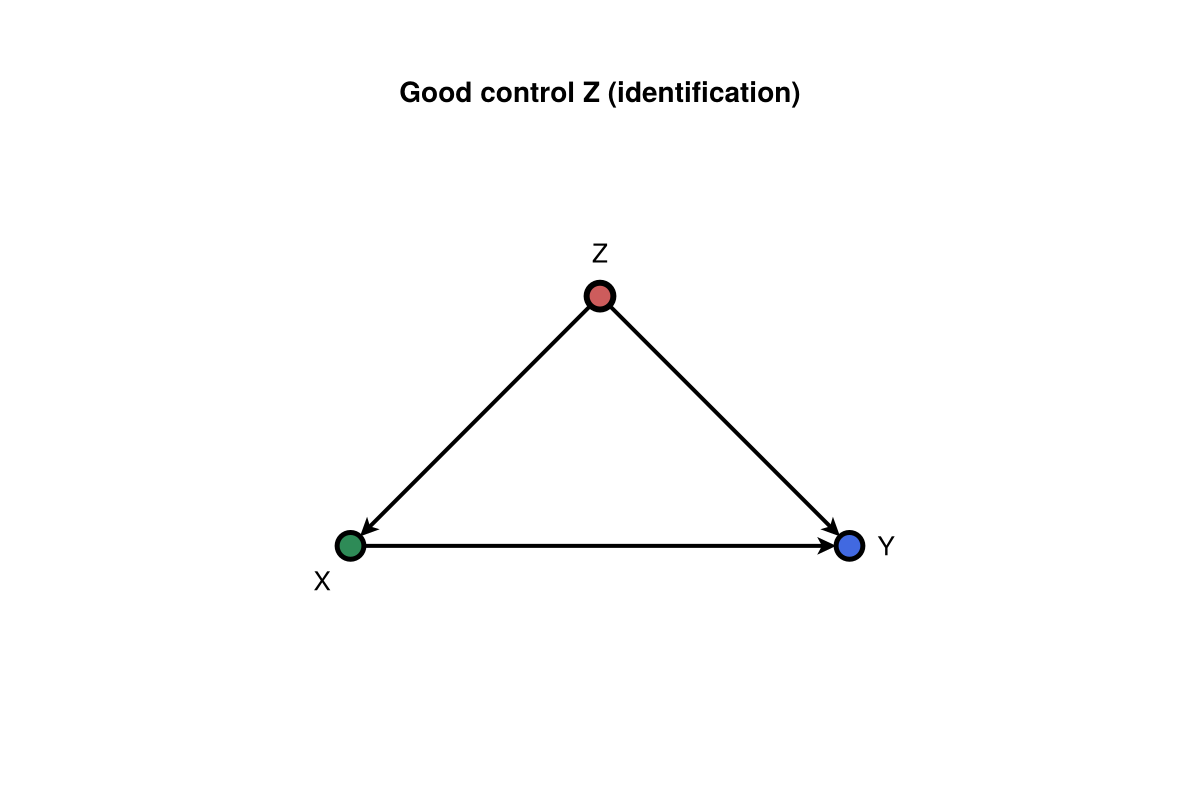

Graph (backdoor paths). Biased paths through Z blocked by adjustment.

adj = backdoor_adjustment_set(g, 2, 3)
fig, _, _ = dagplot_backdoor(g, 2, 3;
    adjustment = adj,
    labels = ["Z", "X", "Y"],
    title = "Backdoor paths (adjust Z)",
)
fig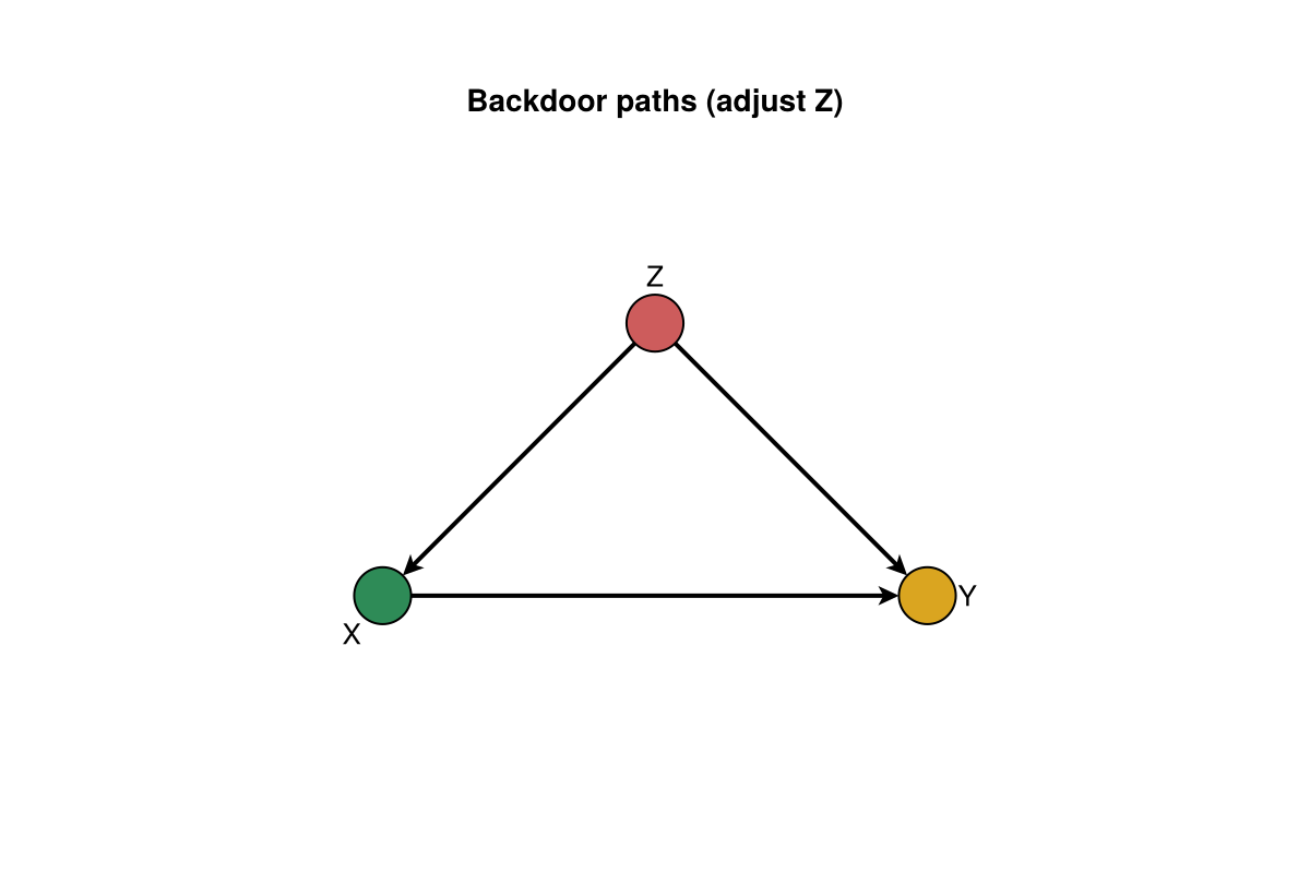

Typed identification. identify returns a certificate-friendly result:

id = identify(g, TotalEffectQuery(:X, :Y); node_names = names)
id.identifiable, id.strategy, id.adjustment

(true, :backdoor, [:Z])

Graph (total effect). Estimand path X → Y only (confounder omitted from the TE diagram).

g_te, _ = chain_graph(["X", "Y"])
fig, _, _ = dagplot_chain(["X", "Y"];
    title = "Total effect path",
)
fig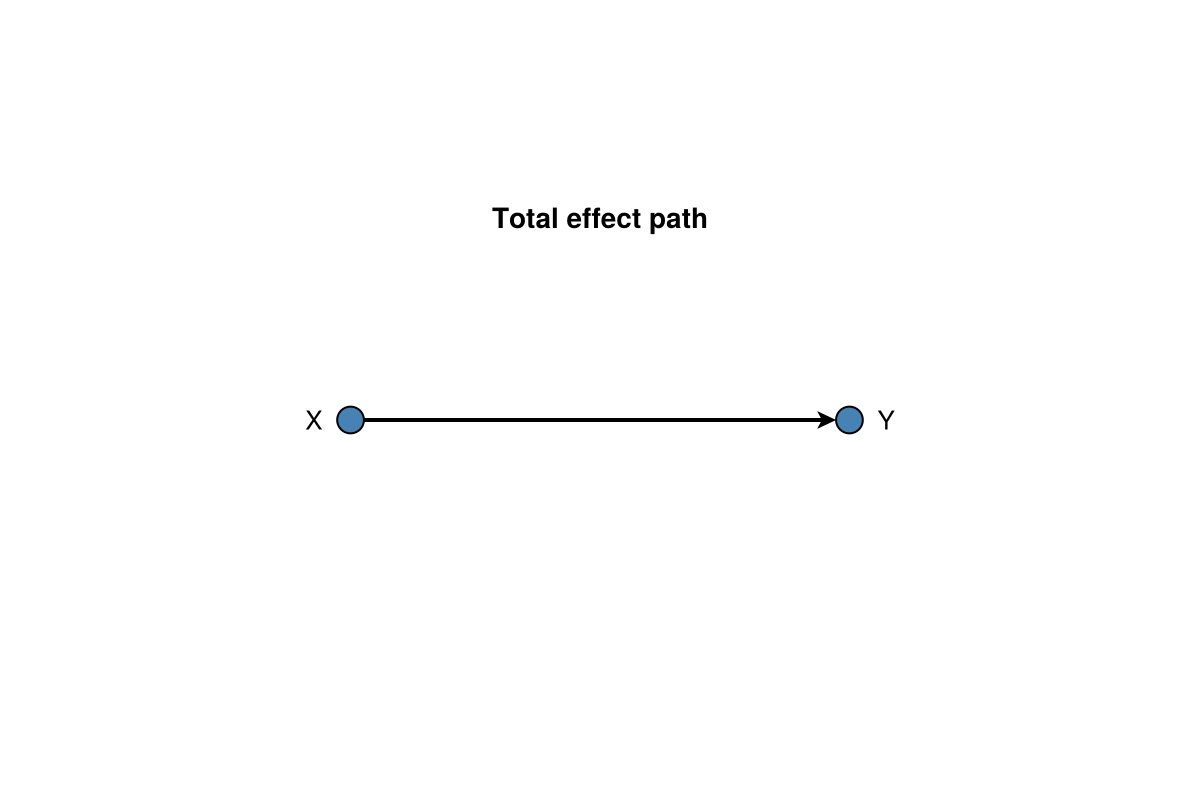

Further reading: Identification API · Graph operations.

2. Mediation (triangle)

Graph. Baseline confounding plus mediator M on A → Y.

using CausalDynamics, Graphs

g = DiGraph(4)
add_edge!(g, 1, 2); add_edge!(g, 1, 3); add_edge!(g, 1, 4)
add_edge!(g, 2, 3); add_edge!(g, 2, 4); add_edge!(g, 3, 4)
names = Dict(1 => :W, 2 => :A, 3 => :M, 4 => :Y)

id = identify(
    g, MediationQuery(:A, :Y, [:M]; effect_kind = :interventional);
    node_names = names,
)
id.identifiable, id.strategy, id.adjustment

(true, :mediation_interventional, [:W])

Graph (identification). Full mediation DAG; adjust W only (M is a mediator, not a good control).

using DAGMakie, CairoMakie

g_id = DiGraph(4)
add_edge!(g_id, 1, 2); add_edge!(g_id, 1, 3); add_edge!(g_id, 1, 4)
add_edge!(g_id, 2, 3); add_edge!(g_id, 2, 4); add_edge!(g_id, 3, 4)
layout_id = [
    Point2f(0.0, 0.0), Point2f(1.2, 0.0), Point2f(2.4, 1.0), Point2f(3.6, 0.0),
]
fig, _, _ = dagplot(g_id;
    layout = layout_id,
    labels = ["W", "A", "M", "Y"],
    color_by = :adjustment,
    exposure = 2,
    outcome = 4,
    adjustment = Set([1]),
    edge_routing = Dict(
        (1, 4) => CurvedEdge(bow = 0.18, side = :right),
        (1, 3) => CurvedEdge(bow = 0.12),
    ),
    title = "Good control W (mediation DAG)",
)
fig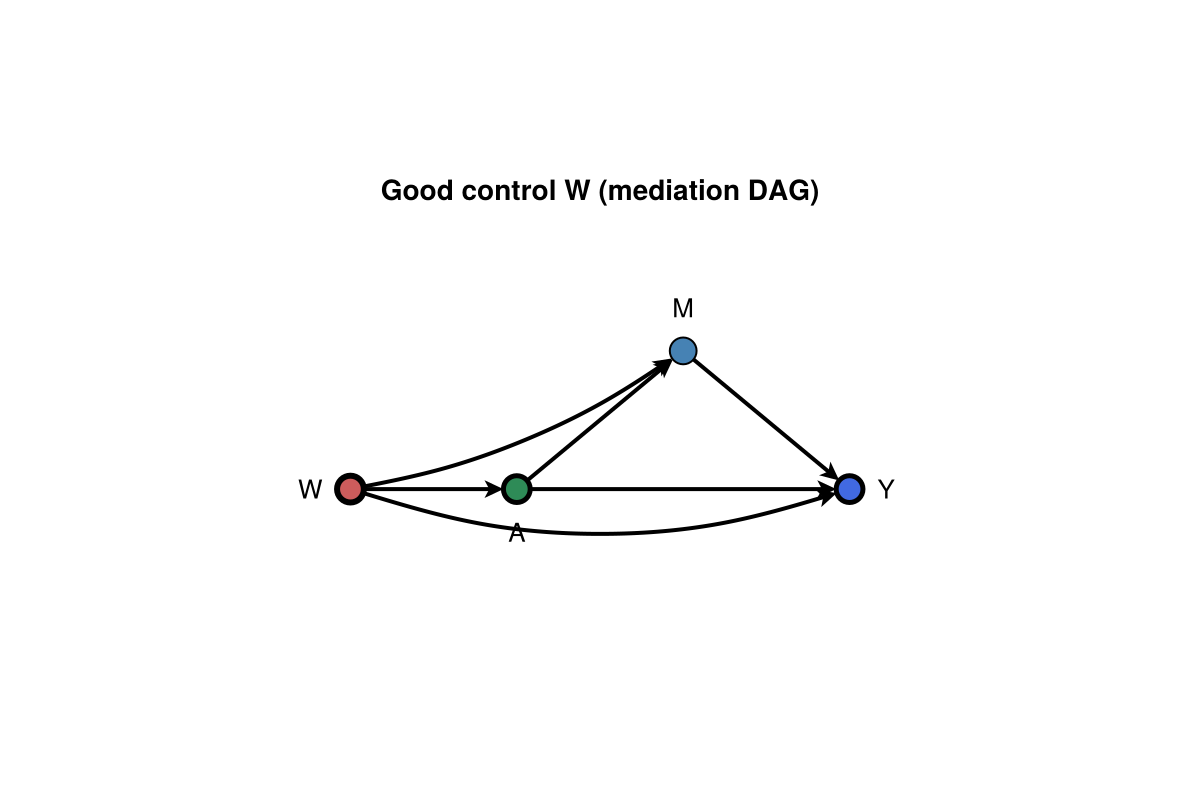

Graph (mediation paths). Direct and indirect routes with W omitted (already adjusted).

fig, _, _ = dagplot_mediation(["A", "M", "Y"];
    title = "Mediation paths (A → M → Y, A → Y)",
)
fig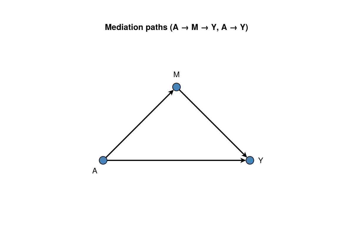

Graph (effect labels). NDE on A → Y, NIE via A → M (illustrative values).

using Graphs: edges, src, dst

g_med, _ = mediation_graph(["A", "M", "Y"])
elookup = Dict((1, 3) => "NDE", (1, 2) => "NIE")
fig, _, _ = dagplot_mediation(["A", "M", "Y"];
    elabels = structural_edge_labels(g_med, [
        get(elookup, (src(e), dst(e)), "") for e in edges(g_med)
    ]),
    elabels_fontsize = 13,
    elabels_distance = 14,
    elabels_rotation = 0,
    title = "Direct and indirect paths",
)
fig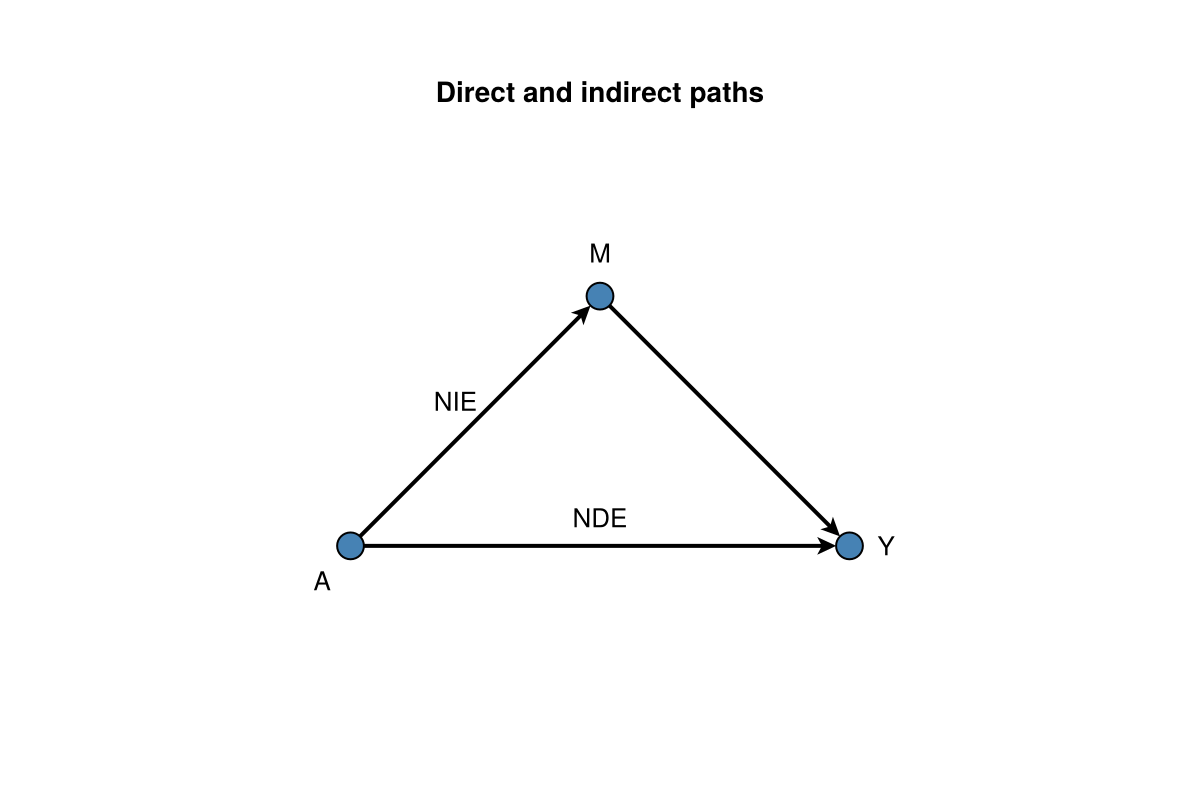

Estimation of interventional NDE/NIE under MTP shifts lives in CausalMediation.jl.

3. Time-indexed graphs

Spec. Two times with baseline w, treatments a, time-varying l, outcome y. The compact TemporalDAGSpec(variables, edges) constructor gives every listed variable default PointwiseSupport (one node per t ∈ 𝒯). For a fixed entity attribute (genotype, site, baseline arm), declare TemporalNodeSpec(...; temporal_support = FromOnsetSupport(onset)) so unrolling keeps one node and panel helpers map to a bare column. Ontological character, when claimed, is declared on a shared ReferentSpec and does not change node count (#29).

using CausalDynamics
using CausalDynamics: TemporalDAGSpec, LaggedEdge, unroll_temporal_dag, TemporalEffectQuery

spec = TemporalDAGSpec([:w, :a, :l, :y], [
    LaggedEdge(:w, :a, 0),
    LaggedEdge(:a, :l, 0),
    LaggedEdge(:l, :a, 1),
    LaggedEdge(:a, :y, 0),
    LaggedEdge(:a, :y, 1),
    LaggedEdge(:w, :y, 0),
])
u = unroll_temporal_dag(spec, 2)
tq = TemporalEffectQuery(:a, :y, 1, 2)
id = identify(u, tq)
id.strategy, id.adjustment

(:temporal_backdoor, [:l, :w])

Graph (identification). Good control w[1] on the unrolled DAG.

using DAGMakie, CairoMakie
using CausalDynamics: temporal_node

w1 = temporal_node(u, :w, 1)
a1 = temporal_node(u, :a, 1)
l1 = temporal_node(u, :l, 1)
a2 = temporal_node(u, :a, 2)
y2 = temporal_node(u, :y, 2)
fig, _, _ = dagplot_temporal(u;
    dx = 2.4,
    dy = 1.7,
    figure_size = (720, 420),
    fit_node_size_to_labels = false,
    color_by = :adjustment,
    exposure = a2,
    outcome = y2,
    adjustment = Set([w1]),
    edge_routing = Dict(
        (a1, y2) => CurvedEdge(bow = 0.14, side = :right),
        (l1, a2) => CurvedEdge(bow = 0.12),
    ),
    title = "Good control w[1] (identification)",
)
fig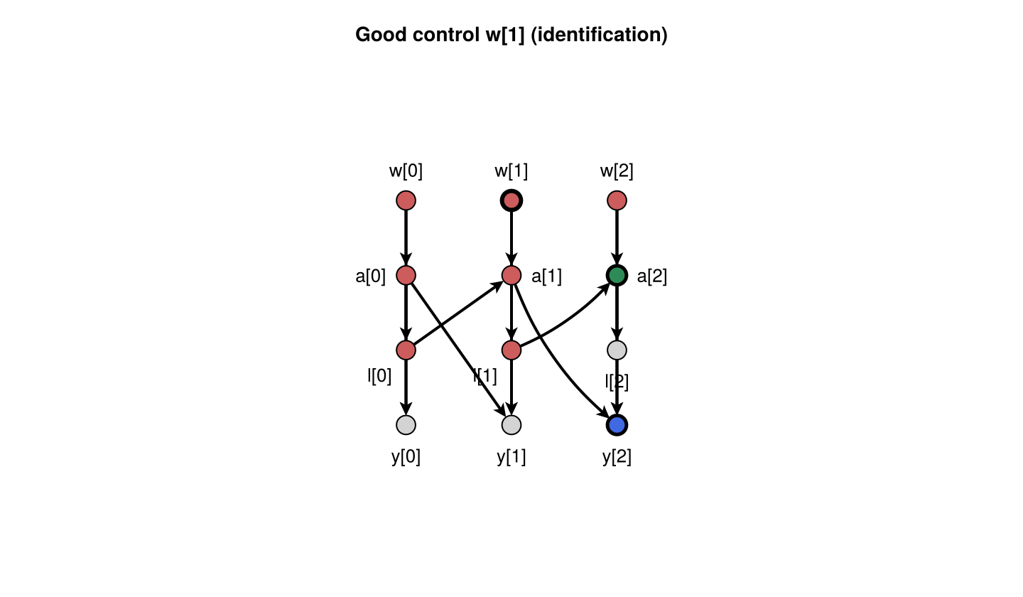

Sequential LMTP estimation: CausalTargeted getting started.

From-onset attributes and glyphs

Support alone fixes node count. A pasture assignment that begins at onset keeps one reused node; its glyph is still a circle unless you declare value_representation = :interval_summary. Optional ontology lives on a shared ReferentSpec, never on the node constructor.

using CausalDynamics
using CausalDynamics: TemporalDAGSpec, TemporalNodeSpec, LaggedEdge, unroll_temporal_dag,
    FromOnsetSupport, PointwiseSupport, ReferentSpec, single_node
using DAGMakie, CairoMakie

sheep = ReferentSpec(:sheep; identity_criterion = :administrative_identifier)
spec = TemporalDAGSpec(;
    nodes = [
        TemporalNodeSpec(:diagnosis; temporal_support = PointwiseSupport(),
            value_representation = :event),
        TemporalNodeSpec(:pasture; temporal_support = FromOnsetSupport(0),
            value_representation = :attribute, referent = sheep),
        TemporalNodeSpec(:burden_summary; temporal_support = PointwiseSupport(),
            value_representation = :interval_summary),
    ],
    edges = [
        LaggedEdge(:diagnosis, :pasture, 0),
        LaggedEdge(:pasture, :burden_summary, 0),
    ],
)
u = unroll_temporal_dag(spec, 0)  # 𝒯 = {0}: one pointwise node each for diagnosis / burden
fig, _, p = dagplot_temporal(u;
    figure_size = (560, 280),
    fit_node_size_to_labels = false,
    title = "Attribute circle vs interval-summary glyph",
)
pasture_i = single_node(u, :pasture)
burden_i = findfirst(k -> first(k) === :burden_summary, u.index_node)
(
    nv(u.graph),
    p[:node_marker][][pasture_i] == :circle,
    p[:node_marker][][burden_i] == interval_summary_node_marker(),
)

(3, true, true)

Further reading: Time-indexed graphs · Terminology.

4. CausalDynamics plot façades

Optional helpers wrap DAGMakie when you already hold node indices from backdoor_adjustment_set:

using CausalDynamics, Graphs, DAGMakie, CairoMakie

g = DiGraph(3)
add_edge!(g, 1, 2); add_edge!(g, 1, 3); add_edge!(g, 2, 3)
plot_backdoor_paths(g, 2, 3; node_labels = ["Z", "X", "Y"])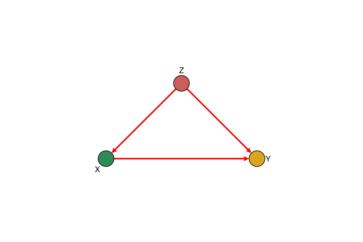

Highlight a chosen adjustment set explicitly:

plot_with_adjustment_set(g, 2, 3, [1]; node_labels = ["Z", "X", "Y"])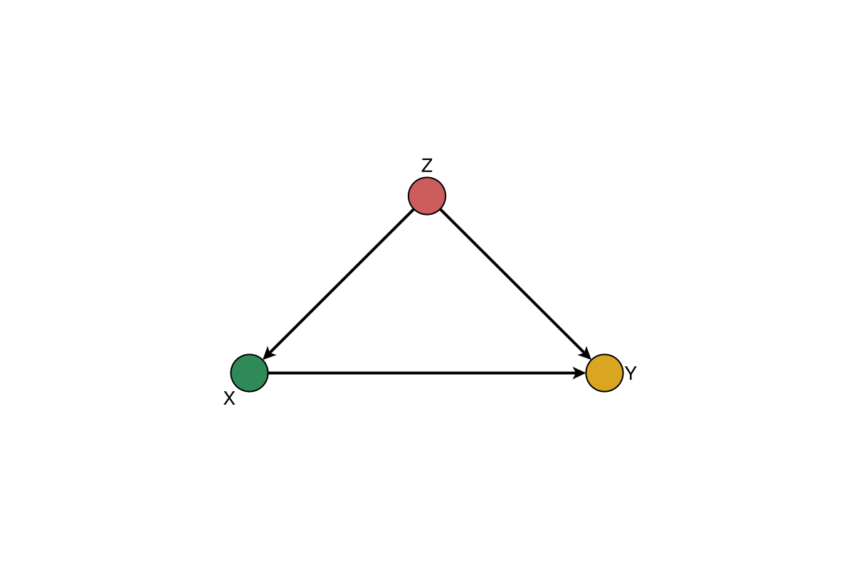

Layout and styling conventions: DAGMakie user guide.

5. SCM simulation and intervention

simulate_scm evaluates each structural equation with parent values in sorted inneighbors order, followed by that node's exogenous draw U. When several parents exist, match the function argument order to ascending parent node indices (e.g. for $Z\to Y$ and $X\to Y$, use (z, x, u) -> …, not (x, z, u)).

equations = Dict{Int, Function}(
    1 => (u,) -> u,
    2 => (z, u) -> z + u,
    3 => (z, x, u) -> 2x + z + u,
)
scm = GraphSCM(g, equations, Set{Int}())
U = Dict(1 => 1.0, 2 => 0.5, 3 => -0.3)
y_factual = simulate_scm(scm, U)
y_do = simulate_scm(apply_intervention(scm, do_intervention(2, 10.0)), U)

Shared-U counterfactuals and discrete-time CDMs: SCM API · Discrete-time CDMs.

6. Nested units (hierarchical $U$)

When farms, herds, or classrooms share a latent draw, put that structure in the generative model, then estimate with ordinary IF tools (optionally cluster-robust in CausalTargeted). CausalDynamics does not fit LMMs.

using CausalDynamics, Random, Statistics

cols, truth = simulate_hierarchical_intercept_ate(
    800; n_clusters = 20, σ_cluster = 1.0, β_a = 0.6, σ_y = 0.3,
    rng = Xoshiro(7),
)
# OLS Y ~ 1 + A + W recovers β_a when U_j is nested noise independent of (A, W)
X = [ones(length(cols[:Y])) cols[:A] cols[:W]]
β̂ = X \ cols[:Y]
isapprox(β̂[2], truth.ate; atol = 0.08)

true

DAG unrolling with plate-style node names: unroll_hierarchical_dag. Cluster sandwich for repeated-outcome MSM: CausalTargeted cluster=. Stress: Hierarchical nesting stress.