CausalTargeted.jl

CausalTargeted implements cross-fitted targeted estimators for continuous and longitudinal exposures, including longitudinal modified treatment policies (LMTP), repeated-outcome profiles, parametric regression standardisation, positivity diagnostics, and omitted-confounder sensitivity. Defaults favour small-to-moderate sample sizes.

Mediation (TE / NDE / NIE, moc, nested Monte Carlo stability) lives in CausalMediation.jl (using CausalMediation). This package supplies Super Learner and LMTP infrastructure that Mediation reuses.

Identification is delegated to CausalDynamics.jl. This package estimates parameters once a query and adjustment set are known.

For longitudinal policy work, CausalDynamics supplies the temporal specification and its edge provenance, while CausalTargeted consumes the resulting panel and declared policy estimand. A policy that persists as one decision rule while its treatment output varies with history should keep that identity in provenance; repeated applications are not independent policy instances. temporal_edge_records is therefore useful for the hand-off and audit trail, but is not an estimator input by itself.

Compared with R and Python

Choose CausalTargeted for Julia-native grids with typed hand-off from IdentificationResult. Prefer lmtp / Ananke when the rest of the pipeline is already R or Python. Details: Comparison · ECOSYSTEM_COMPARISON.md.

Related packages

Design notes: DESIGN.md · NAMING.md · BOUNDARIES.md · ecosystem principles.

Methods and literature

• Getting started — executable walk-throughs (LMTP, mediation, sequential, missingness)
• Comparison — Julia vs R (lmtp, crumble) and Python (Ananke, DoubleML)
• Methods and literature — LMTP, mediation, Super Learner, positivity, sensitivity
• Missingness — Observable policies, certificates, posterior imputation
• Small-n checklist — defaults for tens to low hundreds of units
• Stress validation — catalogued datasets, papers, packages, smoke freeze
• Missingness grid stress — Structural / Dynamical / Observable ledger
• Quarto notebook: docs/stress/stress_validation.qmd — dataset analyses, expected vs actual, DAGMakie / MTP figures
• References — bibliographic list with DOIs

Canonical sources include Díaz et al. (2023) on LMTP; Díaz & Hejazi (2020) and Liu et al. (2024) on stochastic / modern mediation; van der Laan & Rose on TMLE / Super Learner; and Cinelli & Hazlett (2020) on partial-R² sensitivity. BibTeX keys such as diaz2023lmtp live in the CDCS book references.bib.

Quick start

For step-by-step walk-throughs (identify → LMTP, mediation, sequential LMTP, missing data, positivity), see Getting started.

Point-treatment LMTP under baseline confounding uses the DAG below (W → A → Y, W → Y). Identification sets come from CausalDynamics; figures use the optional DAGMakie bridge.

using CausalTargeted, CausalDynamics, Graphs, DAGMakie, CairoMakie

g = DiGraph(3)
add_edge!(g, 1, 2)  # W → A
add_edge!(g, 1, 3)  # W → Y
add_edge!(g, 2, 3)  # A → Y

fig = plot_backdoor_paths(g, 2, 3; node_labels = ["W", "A", "Y"])
fig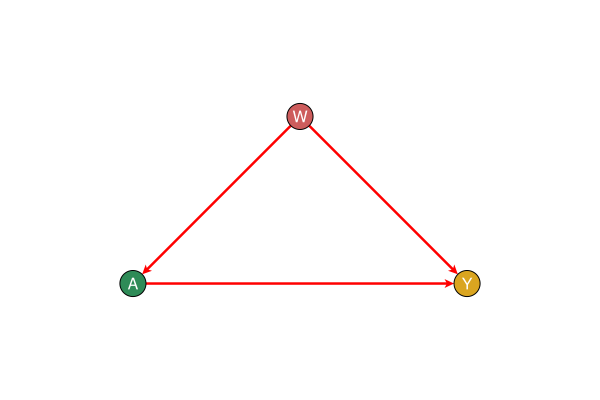

df, _ = simulate_linear_mtp(200)
opts = recommend_run_options(size(df, 1); engine = :lmtp)
δ = collect(-1.0:0.25:1.0)
grid = run_lmtp_grid(
    df, :A, :Y;
    baseline = [:W],
    deltas = δ,
    folds = opts.folds,
    learners_outcome = opts.learners_outcome,
    learners_trt = opts.learners_trt,
    parallel = false,
    positivity = opts.positivity,
    simultaneous = false,
)

fig, ax = plot_mtp_curve(
    grid;
    title = "LMTP grid (synthetic linear MTP)",
    xlabel = "δ (z-scale shift)",
    ylabel = "TE estimate",
)
fig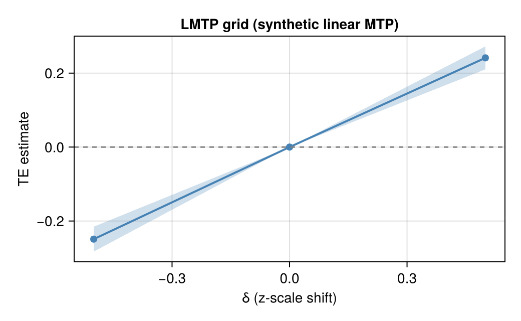

Installation

using Pkg
Pkg.add("CausalTargeted")
# Pkg.develop(path="<path-to-local-clone>")
using CausalTargeted

See also

Worked examples appear in the CDCS book and in application repositories. Prefer package APIs over copying application column names.