Causal highlighting
DAGMakie highlights paths and adjustment sets that you already computed. Identification algorithms live in CausalInference.jl (or CausalDynamics.jl façades). Pass the resulting sets into the plot helpers — the core package does not pull CausalInference (registry CausalInference is incompatible with GraphMakie 0.6).
using Graphs, DAGMakie, CairoMakie

g, labels = confounding_graph(["Z", "X", "Y"])

# From CausalInference.find_min_backdoor_adjustment(g, 2, 3) — or hard-code Z
adjustment = Set([1])

fig, ax, p = dagplot_backdoor(g, 2, 3; adjustment = adjustment, nlabels = labels)
fig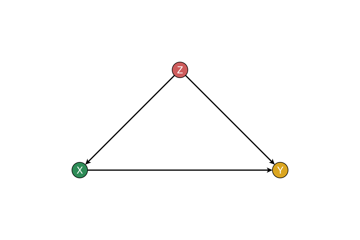
dagplot_adjustment accepts an explicit set the same way:
using Graphs, DAGMakie, CairoMakie

g, labels = confounding_graph(["Z", "X", "Y"])
fig, ax, p = dagplot_adjustment(g, 2, 3; adjustment = Set([1]), nlabels = labels)
fig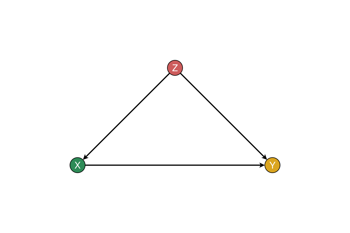
Smart / dagitty-style colours
Pass smart=true (or :ancestors) with treatment and outcome to colour nodes like dagitty “highlight ancestors”. Variables outside the ancestral closure of exposure ∪ outcome are grayed out; shared ancestors (often on backdoors) are marked in red.
| Colour | Role |
|---|---|
| Seagreen | Exposure |
| Royal blue | Outcome |
| Medium seagreen | Ancestor of exposure only |
| Steel blue | Ancestor of outcome only |
| Indian red | Ancestor of both |
| Light gray | Outside the ancestral closure |
Ancestor sets use CausalInference.jl when it is loaded; otherwise Graphs reverse-BFS. smart=:adjustment also thickens a backdoor adjustment set (needs CausalInference, or pass adjustment=).
Default vs smart (confounding triangle)
Same graph, plain steel-blue nodes versus dagitty-style roles. Here $Z$ is an ancestor of both exposure $X$ and outcome $Y$ (indian red).
using Graphs, DAGMakie, CairoMakie

g, labels = confounding_graph(["Z", "X", "Y"])

fig = with_theme(dag_theme()) do
    fig = Figure(size = (900, 360))
    ax1 = Axis(fig[1, 1], title = "Default")
    ax2 = Axis(fig[1, 2], title = "smart = true")
    dagplot!(ax1, g; nlabels = labels)
    dagplot!(ax2, g; smart = true, treatment = 2, outcome = 3, nlabels = labels)
    fig
end
fig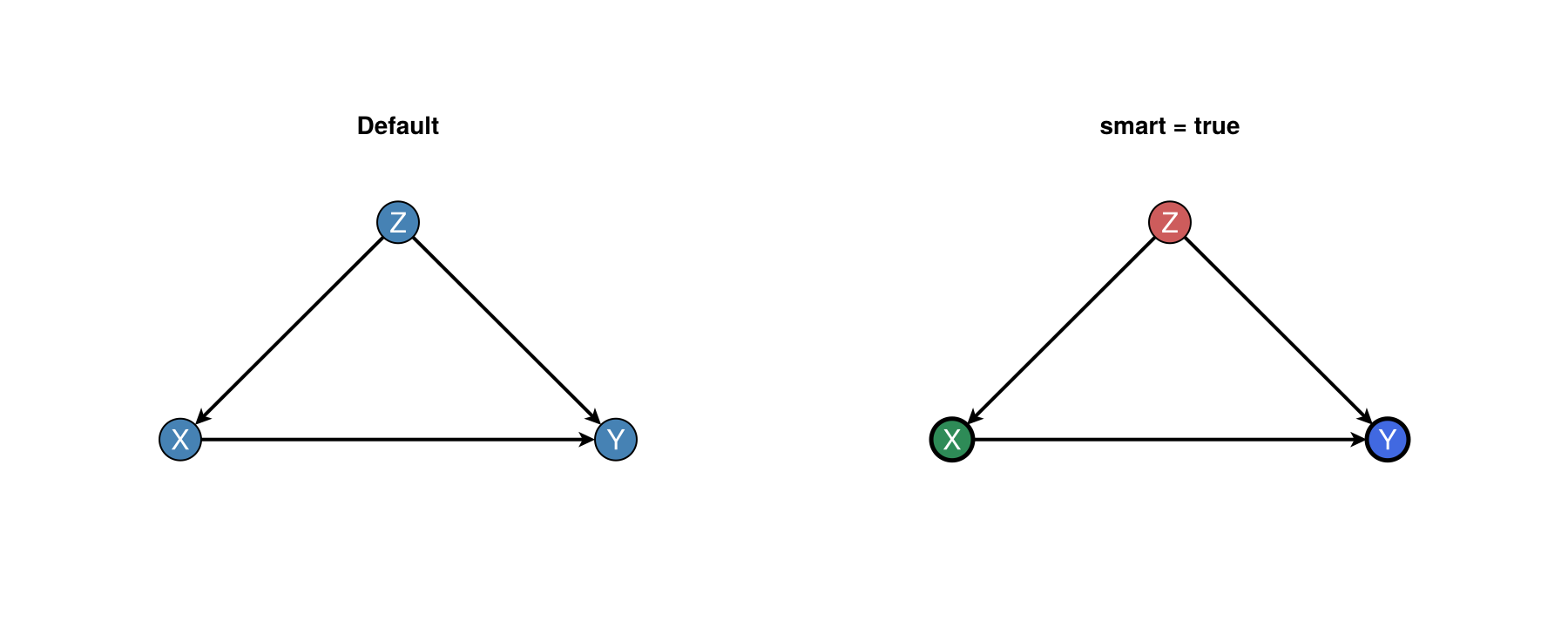
Full role palette
A slightly richer DAG shows every smart role at once: $A$ affects only the exposure, $B$ only the outcome, $Z$ both, and $W$ is irrelevant.
using Graphs, DAGMakie, CairoMakie

# A → X ← Z → Y ← B, X → Y; W isolated
g = SimpleDiGraph(6)
add_edge!(g, 1, 4)  # A → X
add_edge!(g, 2, 4)  # Z → X
add_edge!(g, 2, 5)  # Z → Y
add_edge!(g, 3, 5)  # B → Y
add_edge!(g, 4, 5)  # X → Y
labels = ["A", "Z", "B", "X", "Y", "W"]

roles = classify_smart_roles(g, 4, 5)
@show roles

fig = with_theme(dag_theme()) do
    # Place X below the Z→Y chord so A→X and Z→X do not cross it.
    layout = Point2f[
        (0.0, -2.7),  # A
        (0.0, -0.9),  # Z
        (0.0, 0.9),   # B
        (2.6, -2.2),  # X (below Z→Y so parent edges do not cross it)
        (5.2, 0.0),   # Y
        (0.0, 2.7),   # W
    ]
    fig, ax, p = dagplot_smart(g, 4, 5;
        nlabels = labels,
        layout = layout,
        figure_size = (700, 420),
    )
    ax.title = "A: anc. exposure · B: anc. outcome · Z: both · W: irrelevant"
    fig
end
fig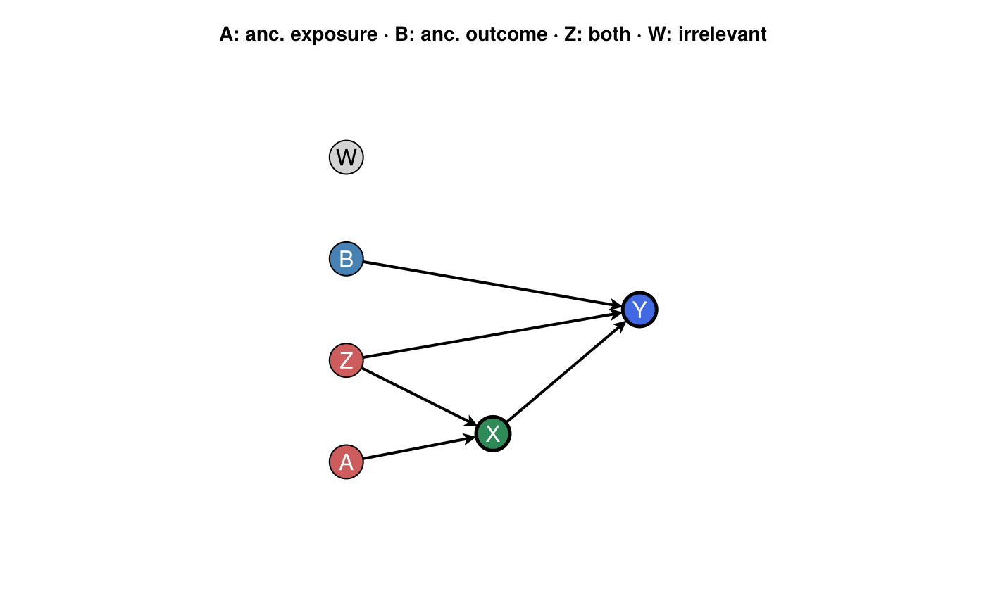
Emphasise an adjustment set
smart=:adjustment keeps the ancestor colours and draws a thicker dark-red outline on adjustment nodes. Pass adjustment= explicitly when CausalInference is not loaded (as in this documentation build).
using Graphs, DAGMakie, CairoMakie

g, labels = confounding_graph(["Z", "X", "Y"])

fig = with_theme(dag_theme()) do
    fig, ax, p = dagplot(g;
        smart = :adjustment,
        treatment = 2,
        outcome = 3,
        adjustment = Set([1]),  # Z
        nlabels = labels,
    )
    ax.title = "smart = :adjustment (Z emphasised)"
    fig
end
fig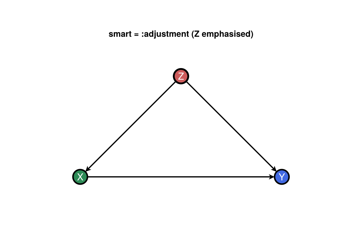
With CausalInference available in your environment you can omit adjustment and let the extension compute a minimal backdoor set:
using CausalInference  # activates DAGMakieCausalInferenceExt
fig, ax, p = dagplot(g; smart = :adjustment, treatment = 2, outcome = 3, nlabels = labels)
That call draws the same emphasis as below (for this DAG the extension returns ${Z}$). The documentation environment does not load CausalInference (registry builds pin GraphMakie incompatible with 0.6), so the figure uses the equivalent explicit set:
using Graphs, DAGMakie, CairoMakie

g, labels = confounding_graph(["Z", "X", "Y"])

fig = with_theme(dag_theme()) do
    fig, ax, p = dagplot(g;
        smart = :adjustment,
        treatment = 2,
        outcome = 3,
        adjustment = Set([1]),  # same as find_min_backdoor_adjustment(g, 2, 3)
        nlabels = labels,
    )
    ax.title = "smart = :adjustment (Z from backdoor set)"
    fig
end
fig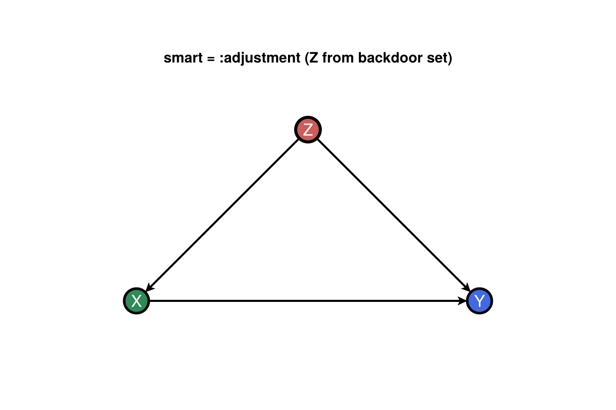
d-Separation titles
Pass separated from dsep / d_separated for axis titles. Use a fork $X ← Z → Y$ (no direct $X → Y$): conditioning on $Z$ d-separates $X$ and $Y$. A confounding triangle with $X → Y$ keeps them d-connected.
using Graphs, DAGMakie, CairoMakie

g, labels = fork_graph(["X", "Z", "Y"])  # X ← Z → Y
# X ⊥ Y | Z (Z blocks the only path)
fig, ax, p = dagplot_dsep(g, 1, 3, Set([2]); separated = true, nlabels = labels)
fig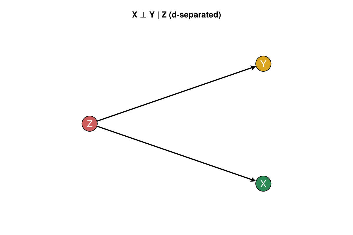
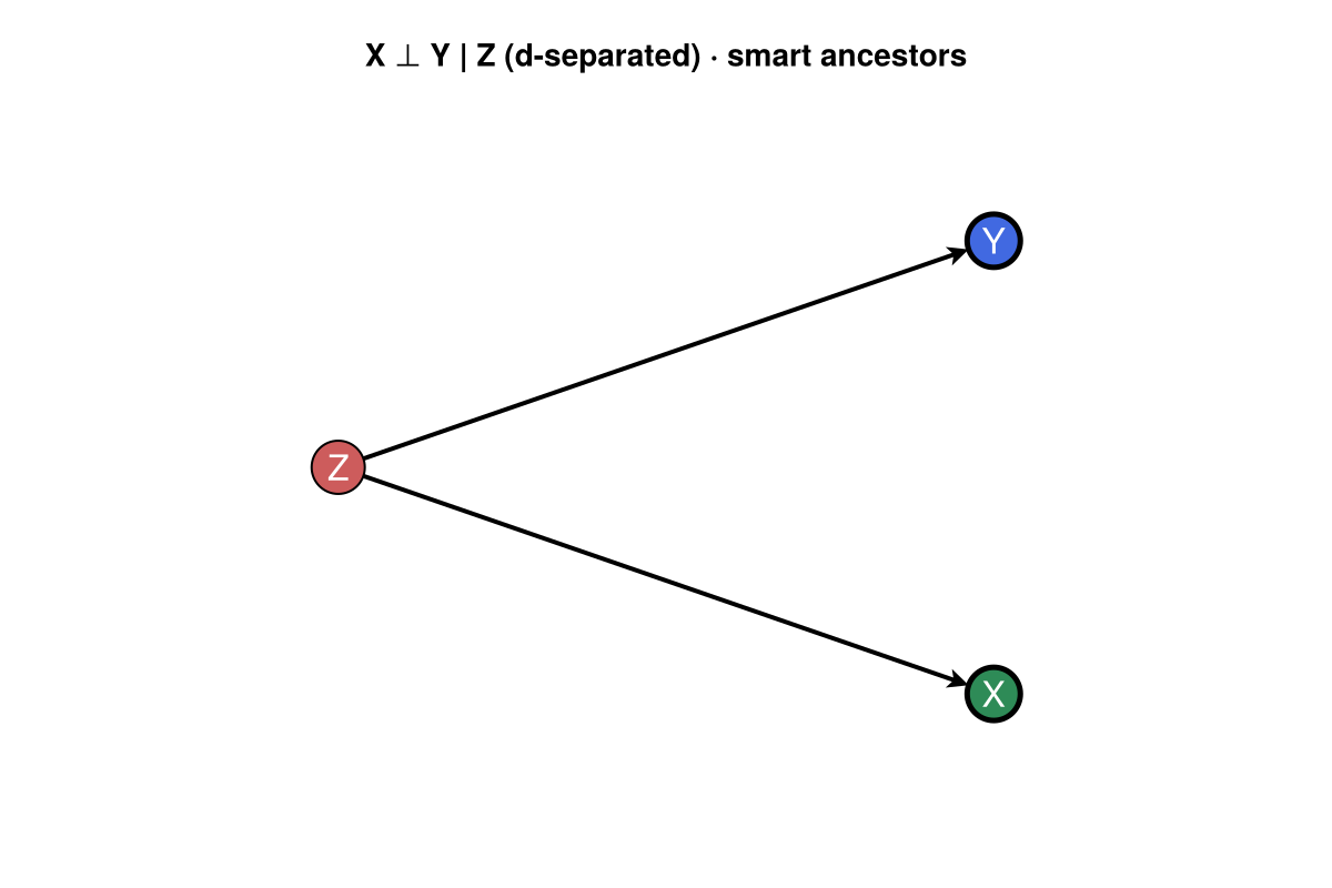
Combine smart colours with a d-separation title when teaching forks:
using Graphs, DAGMakie, CairoMakie

g, labels = fork_graph(["X", "Z", "Y"])
fig = with_theme(dag_theme()) do
    fig, ax, p = dagplot(g;
        smart = true,
        treatment = 1,
        outcome = 3,
        nlabels = labels,
    )
    ax.title = "X ⊥ Y | Z (d-separated) · smart ancestors"
    fig
end
fig