18  Intervening in Stochastic Systems

Status: Draft

v0.4

18.1 Introduction

This chapter shows how to intervene in stochastic dynamical systems, modifying SDEs through the \(do(\cdot)\) operator and evaluating policies under uncertainty. This is part of Doing in the Dynamical stratum, how can we intervene/modify stochastic dynamic processes?

18.2 Interventions in SDEs

18.2.1 The Intervention Operator

When we intervene \(do(A_t = a)\) in a stochastic system, we modify the structural equation for \(A_t\):

\[ A_t \coloneqq a \quad \text{(instead of } \pi(H_t, U^A_t) \text{)} \]

This structural change propagates through the SDE system, and we must account for uncertainty.

18.2.2 How Interventions Modify Stochastic Dynamics

Steps:

1. Set intervention: \(do(A_t = a)\) for all \(t\) in intervention period
2. Modify SDE: Replace \(A_t\) with constant \(a\) in the SDE
3. Solve SDE: Integrate the modified system forward (Monte Carlo simulation)
4. Account for uncertainty: Propagate noise through the system
5. Observe effects: How does the system evolve under intervention (with uncertainty)?

18.2.3 Example: Treatment in Stochastic Compartment Model

Consider a stochastic compartment model with treatment intervention:

\[ \begin{aligned} dS_t &= (-\beta S_t I_t - \alpha \cdot do(A_t = 1)) dt + \sigma_S dW^S_t \\ dI_t &= (\beta S_t I_t - \gamma I_t) dt + \sigma_I dW^I_t \\ dR_t &= (\gamma I_t + \alpha \cdot do(A_t = 1)) dt + \sigma_R dW^R_t \end{aligned} \]

Under intervention \(do(A_t = 1)\), treatment rate \(\alpha\) is applied, but we must account for stochastic noise.

18.2.4 Implementation: Intervention in SDEs

We can implement interventions in SDEs using StochasticDiffEq.jl. Here’s an example:

# Find project root and include ensure_packages.jl
project_root = let
    current = pwd()
    while !isfile(joinpath(current, "Project.toml")) && !isfile(joinpath(current, "_quarto.yml"))
        parent = dirname(current)
        parent == current && break
        current = parent
    end
    current
end
include(joinpath(dirname(Base.active_project()), "scripts", "book_bootstrap.jl"))

@auto_using StochasticDiffEq OrdinaryDiffEq Random Statistics CairoMakie

Random.seed!(42)

# Stochastic compartment model parameters
β = 0.3  # Transmission rate
γ = 0.1  # Recovery rate
α = 0.05  # Treatment rate (when intervention is active)
σ_S = 0.02  # Noise in S
σ_I = 0.02  # Noise in I
σ_R = 0.02  # Noise in R

# Original SDE (no intervention)
function f_original!(du, u, p, t)
    """SIR SDE drift: Susceptible → Infected → Recovered."""
    S, I, R = u
    du[1] = -β * S * I  # dS/dt
    du[2] = β * S * I - γ * I  # dI/dt
    du[3] = γ * I  # dR/dt
end

function g_original!(du, u, p, t)
    """SIR SDE diffusion: additive noise in each compartment."""
    du[1] = σ_S  # Noise in S
    du[2] = σ_I  # Noise in I
    du[3] = σ_R  # Noise in R
end

# SDE under intervention do(A = 1) (treatment active)
function f_intervened!(du, u, p, t)
    """SIR SDE drift with treatment intervention: do(A = 1)."""
    S, I, R = u
    # Intervention: do(A = 1) means treatment is active
    du[1] = -β * S * I - α  # dS/dt: treatment moves S → R
    du[2] = β * S * I - γ * I  # dI/dt: unchanged
    du[3] = γ * I + α  # dR/dt: treatment adds to recovered
end

function g_intervened!(du, u, p, t)
    """SIR SDE diffusion: noise structure unchanged under intervention."""
    # Noise structure unchanged
    du[1] = σ_S
    du[2] = σ_I
    du[3] = σ_R
end

# Initial conditions
u0 = [0.99, 0.01, 0.0]
tspan = (0.0, 50.0)

# Solve original SDE (single trajectory)
prob_original = SDEProblem(f_original!, g_original!, u0, tspan)
sol_original = solve(prob_original, EM(), dt=0.1)

# Solve intervened SDE (single trajectory)
prob_intervened = SDEProblem(f_intervened!, g_intervened!, u0, tspan)
sol_intervened = solve(prob_intervened, EM(), dt=0.1)

# Monte Carlo simulation for uncertainty quantification
n_sims = 100
trajectories_original = []
trajectories_intervened = []

for i in 1:n_sims
    sol_o = solve(prob_original, EM(), dt=0.1)
    sol_i = solve(prob_intervened, EM(), dt=0.1)
    push!(trajectories_original, sol_o)
    push!(trajectories_intervened, sol_i)
end

# Compare expected outcomes
final_I_original = mean([traj.u[end][2] for traj in trajectories_original])
final_I_intervened = mean([traj.u[end][2] for traj in trajectories_intervened])
std_I_original = std([traj.u[end][2] for traj in trajectories_original])
std_I_intervened = std([traj.u[end][2] for traj in trajectories_intervened])

println("Expected final infection rate (mean ± std):")
println("  Original: ", round(final_I_original, digits=3), " ± ", round(std_I_original, digits=3))
println("  Intervened (do(A=1)): ", round(final_I_intervened, digits=3), " ± ", round(std_I_intervened, digits=3))
println("  Reduction: ", round((1 - final_I_intervened/final_I_original) * 100, digits=1), "%")

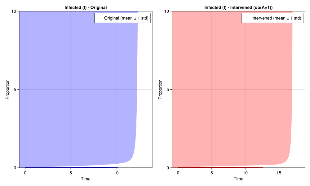
Expected final infection rate (mean ± std):
  Original: -Inf ± NaN
  Intervened (do(A=1)): -Inf ± NaN
  Reduction: NaN%

Figure 18.1: Intervention in stochastic system: comparing original and intervened trajectories with uncertainty

18.3 Policy Evaluation in Stochastic Systems

18.3.1 Evaluating Treatment Policies Under Uncertainty

Question: What is the expected outcome under policy \(\pi\)?

\[ \mathbb{E}[Y^{do(\pi)}] = \mathbb{E}[Y \mid \text{policy } \pi] \]

Method: Simulate SDE under policy (Monte Carlo) and compute expected outcomes over noise realisations.

18.3.2 Uncertainty Propagation

Under interventions, uncertainty propagates:

• Initial condition uncertainty: Affects entire trajectory
• Process noise: Affects system evolution
• Measurement uncertainty: Affects observed outcomes

18.3.3 Optimal Control Under Uncertainty

Question: What policy maximises expected outcome under uncertainty?

\[ \pi^* = \arg\max_\pi \mathbb{E}^{do(\pi)}[Y_T] \]

Methods: Stochastic optimal control, dynamic programming under uncertainty.

18.3.4 Implementation: Policy Evaluation Under Uncertainty

We evaluate policies in stochastic systems using Monte Carlo simulation to account for uncertainty:

# Find project root and include ensure_packages.jl
project_root = let
    current = pwd()
    while !isfile(joinpath(current, "Project.toml")) && !isfile(joinpath(current, "_quarto.yml"))
        parent = dirname(current)
        parent == current && break
        current = parent
    end
    current
end
include(joinpath(project_root, "scripts", "ensure_packages.jl"))

@auto_using StochasticDiffEq OrdinaryDiffEq Random Statistics CairoMakie

Random.seed!(42)

# Example: Treatment policy in stochastic disease model
β = 0.2  # Disease progression rate
α = 0.3  # Treatment effectiveness
σ = 0.05  # Process noise

# Policy 1: No treatment
function f_no_treatment!(du, u, p, t)
    """Disease SDE drift: no treatment policy."""
    X = u[1]
    du[1] = β * X
end

function g_no_treatment!(du, u, p, t)
    """Disease SDE diffusion: additive noise."""
    du[1] = σ
end

# Policy 2: Treat if X > 0.5 (threshold policy)
function f_threshold!(du, u, p, t)
    """Disease SDE drift: threshold policy (treat if X > 0.5)."""
    X = u[1]
    A = X > 0.5 ? 1.0 : 0.0
    du[1] = β * X - α * A * X
end

function g_threshold!(du, u, p, t)
    """Disease SDE diffusion: additive noise."""
    du[1] = σ
end

# Policy 3: Always treat
function f_always_treat!(du, u, p, t)
    """Disease SDE drift: always treat policy."""
    X = u[1]
    du[1] = β * X - α * X
end

function g_always_treat!(du, u, p, t)
    """Disease SDE diffusion: additive noise."""
    du[1] = σ
end

u0 = [0.1]
tspan = (0.0, 20.0)

# Monte Carlo evaluation
n_sims = 200
outcomes1 = Float64[]
outcomes2 = Float64[]
outcomes3 = Float64[]

for i in 1:n_sims
    prob1 = SDEProblem(f_no_treatment!, g_no_treatment!, u0, tspan)
    sol1 = solve(prob1, EM(), dt=0.1)
    push!(outcomes1, sol1.u[end][1])
    
    prob2 = SDEProblem(f_threshold!, g_threshold!, u0, tspan)
    sol2 = solve(prob2, EM(), dt=0.1)
    push!(outcomes2, sol2.u[end][1])
    
    prob3 = SDEProblem(f_always_treat!, g_always_treat!, u0, tspan)
    sol3 = solve(prob3, EM(), dt=0.1)
    push!(outcomes3, sol3.u[end][1])
end

# Compare expected outcomes with uncertainty
println("Expected final severity (mean ± std):")
println("  Policy 1 (no treatment): ", round(mean(outcomes1), digits=3), " ± ", round(std(outcomes1), digits=3))
println("  Policy 2 (threshold): ", round(mean(outcomes2), digits=3), " ± ", round(std(outcomes2), digits=3))
println("  Policy 3 (always treat): ", round(mean(outcomes3), digits=3), " ± ", round(std(outcomes3), digits=3))

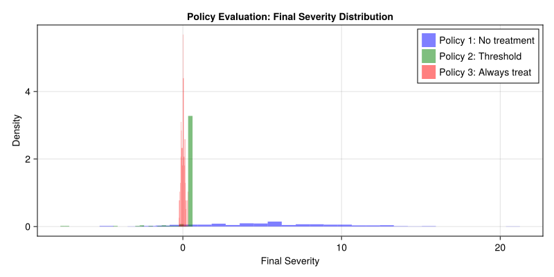
Expected final severity (mean ± std):
  Policy 1 (no treatment): 5.522 ± 4.382
  Policy 2 (threshold): 0.29 ± 0.992
  Policy 3 (always treat): 0.012 ± 0.117

Figure 18.2: Policy evaluation in stochastic systems: comparing policies under uncertainty

18.4 Stratum context

This chapter addresses Doing in the Dynamical stratum: how can we intervene/modify stochastic dynamic processes? Interventions in SDEs modify system dynamics under uncertainty, allowing us to evaluate policies and find optimal control strategies while accounting for stochastic noise.

18.5 Key Takeaways

1. Interventions modify SDEs: \(do(\cdot)\) operator changes stochastic system dynamics
2. Uncertainty propagation: Interventions affect system evolution under uncertainty
3. Policy evaluation: Simulate SDE under policy (Monte Carlo) to evaluate outcomes
4. Optimal control: Find policies that maximise expected outcomes under uncertainty

18.6 Further Reading

• Øksendal (2013): Stochastic Differential Equations
• Stochastic Dynamics: SDEs and Random Processes: SDEs as causal mechanisms
• Advanced Dynamics: Regimes, Networks, and Resilience: Advanced intervention topics
• Policy Evaluation and Dynamic Treatment Strategies: Evaluating policies in stochastic systems

Øksendal, Bernt. 2013. Stochastic Differential Equations: An Introduction with Applications. 6th ed. Springer.