12  From Structure to Time: FEP and Attractors

Status: Draft

v0.3

12.1 Introduction

In the Structural world, we’ve focused on stable modelling assumptions: graph structure, invariances, and abstract relations. This chapter shows how Structural assumptions prepare for time to enter the framework. While still working at an abstract level, we introduce concepts that bridge to the Dynamical world: the Free Energy Principle (FEP) and attractors.

12.2 Structural Summary: What We’ve Learned

12.2.1 What We Learned in Structural

In Part I (Structural), we established:

1. The Causal Hierarchy and Three Strata (Chapter 1): Framework of three worlds and three levels
2. The Primary Unit: The Dyad (Chapter 2): Fundamental unit of directed dependence
3. Pure Structural (Chapter 3): Graph theory, SCMs, identification, do-calculus, counterfactuals, transportability
4. State-Space Models: Inferring structural patterns (perfect forms, invariant mechanisms, edge structure) from observable data (Chapter 12)
5. Observational Methods: Learning from data using G-methods, TMLE, and experimental design (Chapters 19-21)

The Structural world is characterised by:

• Idealised structure: Causal structure expressed as assumptions (e.g., graphs/mechanisms) that are treated as time-invariant within a modelling context
• Invariant Patterns: Stable, environment-independent abstract prehensions
• Graph Structure: Directed dependencies (edges) encoding structural assumptions and invariances
• Abstract Relations: Still no time; relations are abstract, not yet temporal

12.2.2 Idealised and Invariant Attractors in Structural

Idealised attractors (Structural):

• Idealised states toward which a modelled system tends in principle
• Timeless, spaceless
• Represent structure expressed at the level of assumptions (before specifying time-varying dynamics)

Invariant Attractors (Structural):

• Fitness-maximising states that are stable in a fixed environment
• Still abstract, still no time
• Represent invariant mechanisms (stable dependencies across contexts)

Both idealised and invariant attractors belong to the Structural layer: they describe stable targets implied by a model class, before time-varying evolution is made explicit.

12.2.3 Structural Dependencies (Edges)

In the Structural world, edges encode both:

• Idealised structure: Which variables can directly affect which others (model assumptions)
• Invariant patterns: Stable, environment-independent relations (invariances)

Edge structure remains constant, ignoring environments and contexts; edges remain abstract and timeless, not yet temporal.

12.3 The Free Energy Principle as Bridge

12.3.1 FEP Connects Structural to Dynamical Attractors

The Free Energy Principle (FEP) provides a unifying framework that connects Structural (perfect and invariant) to Dynamical (dynamic) attractors (Friston 2010; Friston et al. 2006). Here, optimal, fitness-maximising states are conditional on the environment. Actual occasions prehend their environment, and tend towards (potentially changing) optimal attractors. FEP states that systems minimise variational free energy, which can be understood as:

• Surprise minimization: Systems avoid surprising states
• Prediction error minimization: Systems minimise prediction errors
• Active inference: Systems act to maintain expected states

FEP across worlds:

• Perfect Attractors (Structural): Ideal free energy minima in perfect causal space (perfect edges)
• Invariant Attractors (Structural): Stable free energy minima in structural space (invariant edges)
• Dynamic Attractors (Dynamical): Time-dependent free energy minima (dynamic edges)

12.3.2 FEP as Principle Explaining Edge Evolution

FEP provides the principle that explains why systems tend toward attractor states at all levels, and how edges (prehensive relations) evolve:

• At the Structural level: Edges encode perfect forms and invariant patterns (perfect and invariant prehensive relations)
• At the Dynamical level: Edges encode dynamic equilibria (dynamic prehensive relations)

The FEP shows how the same principle governs edge evolution from Structural to Dynamical, connecting perfect/invariant → dynamic.

12.3.3 The Markov Blanket: System Boundaries in FEP

The Markov blanket is the FEP formalisation of a boundary between organism and environment (Friston 2010, 2013; Whitehead 1978). Each modelled time step is an organism that takes account of (prehends) what is available to it. Environment is not a Newtonian container: it is whatever the step depends on (settled past, contemporaries, exogenous inputs) minus what the model treats as internal. The blanket is the interface through which organism and environment remain distinct yet coupled.

FEP partitions the generative story as follows:

1. Internal states (\(\mu\)): The organism, latent variables the model evolves (e.g. \(X_t\) in a state-space model). Each \(\mu_t\) is the settled state that becomes input for the next step.
2. External states (\(\eta\)): The environment in the strict sense, everything outside the modelled organism whose direct influence is mediated by the blanket (or left unmodelled).
3. Markov blanket (\(s\), \(a\)): The interface:

• Sensory states (\(s\)): What is given in observation (\(Y_t\)), not the full latent process.
• Active states (\(a\)): Actions and interventions (\(A_t\), \(do(\cdot)\)) that fix what may influence transitions.

What endures across time steps (patient identity, invariant graph \(G\), mechanism class, attractor regime) is a society¹ in Whitehead’s sense. Societies stabilise the environment enough for \(\mu ⫫ \eta \mid (s,a)\) to be a useful idealisation.

12.3.4 Conditional Independence Structure

The blanket’s statistical content is conditional independence:

\[ \mu ⫫ \eta \mid (s, a) \]

Once we hold fixed what the organism presents (\(s\)) and what it does (\(a\)), internal and external states are informationally separated. We do not observe \(\eta\) directly; we sense the environment only through \(s\), and act on it only through \(a\). That asymmetry is why data must not be confused with mechanism.

12.3.5 FEP and System Boundaries

The Free Energy Principle states that systems minimise variational free energy by maintaining blanket structure, continuing as organisms with a stable interface to their environments (Friston 2010; Friston et al. 2006). In a CDM, specifying \((f, h, G)\) is partly specifying which society we assume: which defining characteristic links successive time steps.

World context: The Markov blanket is a Structural/Dynamical concept. Structurally, it fixes which relations are invariant (the society’s form); dynamically, it is maintained through time as steps succeed one another.

12.3.6 Connection to Three Levels of Reason

The blanket mediates all three levels of Reason:

• Level 1 (Association / Seeing): Learn from observations, \(P(Y_t \mid Y_{1:t-1})\) and related objects use only \(s\), not full \(\mu\) or \(\eta\).
• Level 2 (Intervention / Doing): \(do(\cdot)\) on \(a\) fixes what the organism may take up, propagating through \(f\) into future \(\mu\).
• Level 3 (Counterfactual / Imagining): Same organism (fixed creative advance \(\mathbf{u}\), Introduction), alternative concrescences under a different action on \(a\).

12.3.7 Summary: process terms and CDM notation

Process term	CDM / FEP role
Organism	Internal \(\mu_t\) (e.g. \(X_t\)); trajectory of occasions under \(f\)
Environment	External \(\eta\); parents and \(U\) outside \(\mu\)
Society	Invariant \(G\), \(F\), attractor, or shared mechanism class across \(t\)
Markov blanket	Sensory \(s\) (\(Y_t\)), active \(a\) (\(A_t\)); \(\mu ⫫ \eta \mid (s,a)\)

A statistical population is not automatically a society: transport and cohort generalisation require a shared defining characteristic (see Transportability). Operational detail appears in State-Space Models and Causal Decision-Making; Concept Reference, Table 4.

12.4 World Comparison: Structural vs Dynamical

Aspect	Structural	Dynamical
Attractor Type	Perfect and Invariant (ideal forms, stable patterns)	Dynamic (changing, environment-dependent)
Nature	Abstract relations, no time	Dynamic processes, time enters
FEP Application	Ideal and stable free energy minima	Time-dependent free energy minima
Mechanisms	Perfect and invariant mechanisms	Time-dependent mechanisms
Examples	Graph structure, perfect forms, invariant patterns	Dynamic processes, flows

12.5 Attractor Progression: Structural → Dynamical

Perfect and Invariant Attractors (Structural):

• Perfect: Ideal forms toward which systems tend in principle
• Invariant: Stable, environment-independent fitness-maximising states
• Both abstract, both no temporal dimension

Dynamic Attractors (Dynamical):

• Time-dependent, environment-dependent
• Fitness-maximising but changing with environment
• Temporal dimension enters

The progression: From perfect and invariant attractors (Structural) to dynamic attractors that change with time and environment (Heraclitean/Whiteheadian process).

12.6 Time Enters: The Dynamical Dimension

12.6.1 What Changes: Structural Prehensive Relations → Temporal Prehensive Relations

With the transition to Dynamical, time enters the framework:

• Structural edges → Dynamic edges: Prehensive relations become time-dependent
• Abstract prehensive relations → Temporal prehensive relations: Relations gain temporal structure
• Perfect/invariant mechanisms → Dynamic mechanisms: Processes evolve over time
• Perfect/invariant attractors → Time-dependent attractors: Attractors shift with environment

12.6.2 Time Enters, But Processes Remain Abstract

Critical distinction: Time enters, but processes remain abstract (not yet material/physical):

• Temporal but abstract: Edge structure becomes time-dependent, but still abstract
• Time-dependent abstract processes: Processes become time-dependent, but not yet actualised into material reality
• Not yet material/physical: The Dynamical world is temporal but abstract, not yet fully embodied

Edge structure becomes temporal, but still abstract:

• Edges encode time-dependent prehensive relations
• Edge mechanisms evolve over time
• But edges remain abstract, not yet material/physical

12.6.3 Structural Edges → Dynamic Edges

The transition in terms of edges:

• Perfect/invariant prehensive relations → Dynamic prehensive relations
• Perfect/invariant edge semantics (ideal forms, stable patterns) → Dynamic edge semantics (time-dependent patterns)
• Timeless but structured → Temporal but abstract

The edges themselves don’t change, what changes is the temporal structure of the edges, from perfect/invariant to dynamic, while remaining abstract.

12.6.4 Heraclitean Change

“Everything flows” (πάντα ῥεῖ) and “you cannot step into the same river twice” (Kirk et al. 1983). The optimum is ever-changing, but this change is still abstract, not yet material/physical actualisation.

This is the key transition: from abstract relations (Structural) to temporal but abstract processes (Dynamical). Full material/physical actualisation happens at the Dynamical → Observable transition.

12.7 Setting Up Part II: Dynamical

In Part II (Dynamical), we will explore:

1. Deterministic Dynamics (ODEs): Dynamic processes as causal mechanisms (dynamic edges)
2. Stochastic Dynamics (SDEs): Time-dependent processes with environmental variation (stochastic edges)
3. Regime Switching: Multiple dynamic attractors (switching edge mechanisms)
4. Network Models: Prehensive structure in space (spatial edge structure)
5. Dynamics on Networks: Collective dynamic attractors (network edge dynamics)
6. Resilience and Robustness: Stability of dynamic attractors (edge stability)

The Dynamical world introduces:

• Time: Temporal dimension enters (edges become time-dependent)
• Dynamic Processes: Time-dependent mechanisms (edge mechanisms evolve over time)
• Dynamic Attractors: Environment-dependent, ever-changing optima (dynamic edge attractors)
• Temporal but Abstract: Processes are time-dependent but still abstract, not yet material/physical

12.7.1 Emphasising Edges in Dynamical World

In the Dynamical world, we will see how:

• Edges become temporal: From perfect/invariant prehensive relations to dynamic prehensive relations
• Edge structure becomes time-dependent: The graph structure evolves over time
• Edge mechanisms are dynamic: The functions encoding prehensive relations change with time
• Edge topology remains abstract: Still abstract, but now temporal

The focus remains on edges (prehensive relations) as the fundamental units, but now they are time-dependent while remaining abstract. Full material/physical actualisation happens at the Dynamical → Observable transition.

12.8 Pedagogical attractors and intervention timing

These examples bridge Attractor Progression to Part II: multistability on a fixed graph, epidemic thresholds under vaccination rollout, and ecosystem health under restoration effort. Each uses the organism–society gloss from The Markov Blanket.

The same interaction graph (who is linked to whom) can still support more than one stable long-run pattern. An ecosystem may sit in a healthy configuration or a degraded one; a regulatory network may settle into two expression regimes. Which pattern appears often depends on where the system starts, not on rewiring the graph (Scheffer et al. 2009; Strogatz 2014). For policy, that distinction matters: some interventions only shake the system within its current pattern; others push it across a threshold into a different attractor (a tipping point).

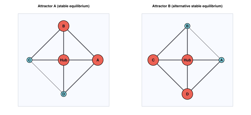
Figure 12.1 is a small pedagogical cartoon: five coupled units on a wheel (hub plus four neighbours), the sort of layout you might sketch for a hub gene and four regulated targets, or a keystone species and four strongly interacting partners. It sits in the spirit of multistable attractor networks on fixed regulatory graphs (Wang et al. 2016).

We can illustrate this by reading each node as a small organism (one unit concrescing in time), what it receives along incoming links as what it prehends from neighbours, and the shared wheel topology plus coupling rule as a society, occasions held together by the same defining characteristic, not simply “five things in a group.” The rim nodes are co-organisms in that society (or population).

We run the same society twice with different starting values:

1. Each unit is pulled toward one of two local tendencies (high or low), think “on/off” or “high/low” expression.
2. Neighbours gently encourage one another to agree (coupling along the wheel).
3. The two runs end in different rim patterns, two stable expression (or abundance) patterns on one wiring diagram.

Node size and colour show how strongly each unit has settled into its role; edge thickness highlights links between strongly settled neighbours. The equations and simulation are in the figure caption and code; the causal lesson is: shared structure, different histories, different equilibria.

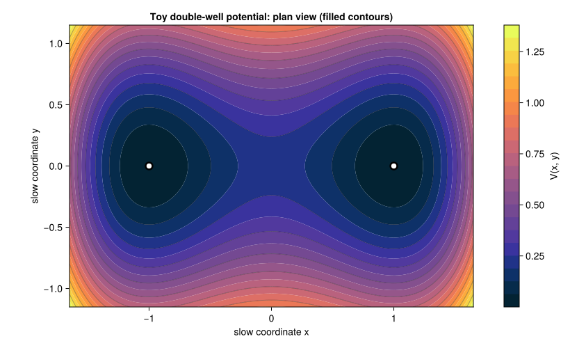
Figure 12.2 gives the same idea as a landscape picture: two valleys (markers) separated by a ridge. Motion tends downhill into one valley or the other, two basins of attraction. The plot is a toy surface for intuition only; it is not the literal energy landscape of the five-node simulation, and many real systems need richer summaries than a single two-dimensional hillscape (Strogatz 2014; Leonov and Kuznetsov 2016). It still makes multistability easy to see: more than one place the dynamics can settle, with a barrier between them.

Figure 12.1: Wheel coupled-units topology (pedagogical; attractor-network motivation (Wang et al. 2016)): two simulated concrescences from \(u_i' = u_i - u_i^3 - \lambda(Lu)_i\); node size and colour show prehensive intensity \(\iota_i = \mathrm{clip}((u_i+1)/2)\) at the superject (terminal state); edge thickness uses \(\max(\iota_i,\iota_j)\).

Figure 12.2: Toy double-well potential \(V(x,y)=0.22(x^2-1)^2+0.55y^2\), shown as filled contours in the \(x\)–\(y\) plane (plan view of the usual basin landscape); overlaid contours mark level sets, and markers sit near the two minima. Gradient flow \(\dot{x}=-\partial V/\partial x\), \(\dot{y}=-\partial V/\partial y\) has stable equilibria in those valleys. A general multistable ODE need not be gradient; high-dimensional systems are often summarised by quasi-potentials (Scheffer et al. 2009; Leonov and Kuznetsov 2016).

12.9 Example: Epidemic thresholds and rollout timing

Achieving herd immunity requires vaccinating a critical threshold of the population (typically 70–90% depending on transmissibility) (Anderson and May 1992; keeling2011modelling?). Below that threshold, an outbreak can grow large before fading; above it, transmission is damped from the start. The generative model below is a weekly SIR compartment model on population fractions: a seeded infection, mass-action transmission, mean infectious period of about ten days (\(\gamma^{-1}\)), and a vaccination campaign that moves susceptibles into \(R\) at a scenario-specific rate (slow vs fast rollout, plus baseline immunity).

First rows of the generative panel (weekly fractions):

Table 12.1

6×10 DataFrame

Row	week	scenario	S	I	R	cumulative_incidence	baseline_immunity	herd_immunity_threshold	peak_infected	final_attack_rate
	Int64	String	Float64	Float64	Float64	Float64	Float64	Float64	Float64	Float64
1	0	slow rollout (~32% immune at t=0)	0.679	0.001	0.32	0.32	0.32	0.740741	0.166693	0.982145
2	1	slow rollout (~32% immune at t=0)	0.677703	0.00176097	0.320536	0.320536	0.32	0.740741	0.166693	0.982145
3	2	slow rollout (~32% immune at t=0)	0.675347	0.00309357	0.321559	0.321559	0.32	0.740741	0.166693	0.982145
4	3	slow rollout (~32% immune at t=0)	0.671254	0.00541152	0.323334	0.323334	0.32	0.740741	0.166693	0.982145
5	4	slow rollout (~32% immune at t=0)	0.664289	0.00939737	0.326313	0.326313	0.32	0.740741	0.166693	0.982145
6	5	slow rollout (~32% immune at t=0)	0.652631	0.0161192	0.331249	0.331249	0.32	0.740741	0.166693	0.982145

Figure 12.3 summarises the two campaigns. With \(R_0 \approx 3.9\) the herd-immunity threshold is \(1 - 1/R_0 \approx 74\%\) immune. The slow rollout scenario peaks at roughly 17% currently infected and an attack rate near 98%; the fast rollout keeps the peak near 0.5%, same epidemic mechanism, different timing and coverage of the intervention.

Figure 12.3: Weekly SIR with vaccination campaign (\(R_0 \approx 3.9\), threshold \(\approx 74\%\) immune): slow vs fast rollout. Top: infected fraction \(I(t)\); bottom: cumulative incidence \(1-S-I\). Dashed line: 10% peak prevalence reference.

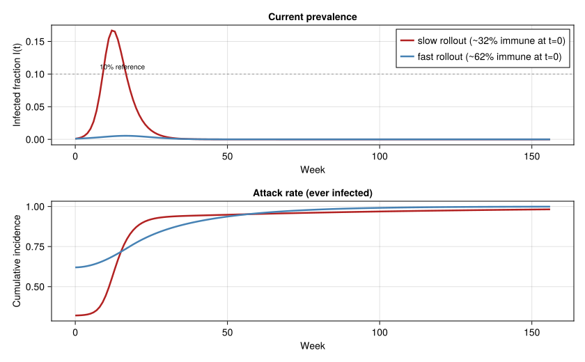
This illustrates how interventions can shift systems between different attractor states: shared epidemic mechanism, different campaign speed and coverage, qualitatively different burden. The transition depends on the intervention threshold, not on rewiring the contact structure.

12.10 Example: Resilience, resistance, and restoration effort

Restoring a degraded ecosystem requires different intervention effort depending on how far the system sits from a healthy attractor. The generative model below tracks an ecosystem health index \(H_t \in [0,1]\) (1 = reference healthy state) on a lake or rangeland slowly stressed by nutrient loading. Intrinsic dynamics are bistable (healthy and degraded basins); restoration effort \(u_t\) (stocking, rewilding, reduced grazing) can push the index across a tipping band near \(H \approx 0.5\).

First rows of the generative panel:

Table 12.2

6×6 DataFrame

Row	year	scenario	health_index	environmental_stress	restoration_effort	tipping_threshold
	Int64	String	Float64	Float64	Float64	Float64
1	1	early + maintenance	0.85	0.000167927	0.062	0.5
2	2	early + maintenance	0.881984	0.000428067	0.062	0.5
3	3	early + maintenance	0.910032	0.000740005	0.062	0.5
4	4	early + maintenance	0.933423	0.00109119	0.062	0.5
5	5	early + maintenance	0.951992	0.00147479	0.062	0.5
6	6	early + maintenance	0.966074	0.00188636	0.062	0.5

Figure 12.4 plots the three scenarios. No restoration declines from \(H_0 \approx 0.85\) toward a degraded basin (about 0.4 by year 70). Early + maintenance (strong effort years 1–22, then light upkeep) holds health near 0.8–0.99. Late intensive effort (from year 29, after health has slipped to \(\approx 0.85\) and would fall further without action) recovers toward 1.0, but only with stronger, longer forcing, illustrating resistance when control is delayed.

Figure 12.4: Ecosystem health \(H_t\) under rising environmental stress (nutrient-loading proxy) and three restoration policies. Dashed line: tipping threshold \(H_c=0.5\). Right axis: stress and effort (scenario with early intervention).

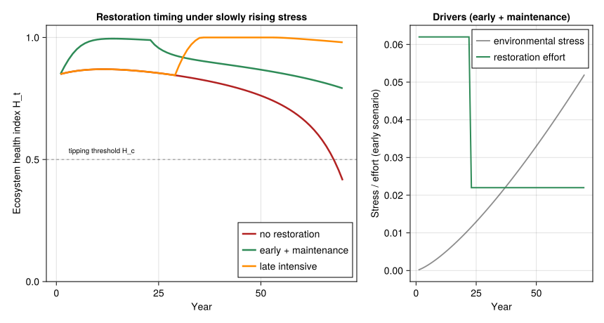
Early intervention (when the state is still reachable with modest effort) differs from reversing a shift after deep degradation, when the same society of processes may require sustained forcing.

12.11 Worked Example: Sheep System Evolving Through Worlds

12.12 Worked Example: Sheep System from Structural to Dynamical

Structural View (Part I):

• Perfect forms: ideal causal structure of predator-prey relations
• Invariant patterns: stable, environment-independent interactions
• Abstract relations: graph structure of interactions
• No time: timeless, spaceless causal structure

Dynamical View (Part II):

• Dynamic mechanisms: time-dependent predator-prey dynamics
• Dynamic attractors: population states that change with environment
• Dynamic processes: actual population trajectories over time

The same system, now with time: from abstract structural relations to dynamic processes.

12.13 Transition to Dynamical

As we move to Part II, we transition from:

• Perfect/invariant mechanisms → Dynamic mechanisms
• Perfect/invariant attractors → Time-dependent attractors
• Abstract relations → Dynamic processes
• No time → Time enters

The Dynamical world introduces the temporal dimension while maintaining causal structure, preparing us for the Observable world where processes become fully actualised. Dynamical is made from Structural, it takes the structural forms (perfect and invariant) and dynamizes them, further embodying the inner worlds.

12.14 World Context

This chapter bridges the Structural and Dynamical worlds. We’ve completed our exploration of structural patterns (perfect forms and invariant patterns) and now introduce the Free Energy Principle and dynamic processes. This sets the foundation for understanding how time enters the framework through gradual embodiment, Dynamical is made from Structural, further embodying the inner worlds. This prepares us for the Dynamical world where dynamic attractors and temporal processes appear.

12.15 Key Takeaways

1. Structural summary: Perfect forms and invariant patterns exist within the Structural world (perfect and invariant edges)
2. Organism–environment–society: Markov blanket as prehensive interface; see The Markov Blanket
3. The Free Energy Principle as bridge: FEP connects Structural (perfect/invariant) → Dynamical (dynamic) attractors (perfect/invariant → dynamic edges)
4. Time enters: Structural prehensive relations (edges) become dynamic prehensive relations (edges)
5. Temporal but abstract: Edge structure becomes time-dependent, but processes remain abstract (not yet material/physical)
6. Actualisation happens later: Full material/physical actualisation happens at Dynamical → Observable transition, not in Dynamical world itself
7. This transition prepares us for Part II: Dynamical

12.16 Further Reading

• Whitehead (1978): Process and Reality: organism, environment, and society (Part II; optional process background)
• Friston (2010): “The free-energy principle: a unified brain theory?”
• Friston et al. (2006): “A free energy principle for the brain”
• The next chapter begins Part II: Dynamical
• See Deterministic Dynamics: ODEs as Causal Processes to continue

Anderson, Roy M., and Robert M. May. 1992. Infectious Diseases of Humans: Dynamics and Control. Oxford University Press.

Friston, Karl. 2010. “The Free-Energy Principle: A Unified Brain Theory?” Nature Reviews Neuroscience 11 (2): 127–38.

Friston, Karl. 2013. “Life as We Know It.” Journal of The Royal Society Interface 10 (86): 20130475.

Friston, Karl, James Kilner, and Lee Harrison. 2006. “A Free Energy Principle for the Brain.” Journal of Physiology-Paris 100 (1–3): 70–87.

Kirk, Geoffrey S., John E. Raven, and Malcolm Schofield. 1983. The Presocratic Philosophers: A Critical History with a Selection of Texts. 2nd ed. Cambridge University Press.

Leonov, Gennady A., and Nikolay V. Kuznetsov. 2016. Hidden Attractors in Dynamical Systems: Systems with No Equilibria, Coexistence of Attractors and Multistability. Lecture slides, Faculty of Mathematics and Mechanics, St. Petersburg University. https://math.spbu.ru/user/nk/PDF/Hidden-attractor-coexistence-multistability.pdf.

Scheffer, Marten, Jordi Bascompte, William A. Brock, et al. 2009. “Early-Warning Signals for Critical Transitions.” Nature 461 (7260): 53–59.

Strogatz, Steven H. 2014. Nonlinear Dynamics and Chaos: With Applications to Physics, Biology, Chemistry, and Engineering. 2nd ed. Westview Press.

Wang, Le-Zhi, Ri-Qi Su, Zi-Gang Huang, et al. 2016. “A Geometrical Approach to Control and Controllability of Nonlinear Dynamical Networks.” Nature Communications 7 (1): 11323. https://doi.org/10.1038/ncomms11323.

Whitehead, Alfred North. 1978. Process and Reality: An Essay in Cosmology. Edited by David Ray Griffin and Donald W. Sherburne. Free Press.

---

1. A society is a nexus of occasions sharing a defining characteristic; what we call a “unit” or “system” is usually a society, not one time step.