3  The Causal Hierarchy and Three Strata

Status: In Progress

v0.4

3.1 Introduction

The Introduction argued that a complex system is a process of becoming, not a static thing, and that scientific models must separate what we observe, what we do, and what we imagine for a specific unit (Whitehead 1978; Pearl 2009). This chapter makes that programme operational. We fix two complementary grids:

1. Three strata: where modelling assumptions live (structure, dynamics, measurement).
2. Three levels of Reason: which causal queries those assumptions support (association, intervention, counterfactual).

The process stance fixes what we model: unfolding systems linked by prehension (taking account of). The strata clarify where assumptions sit. The levels clarify which queries are feasible under those assumptions. What data show is not the same question as what we do to a system; Pearl’s hierarchy makes that separation mathematical (Pearl 2009; Bareinboim 2026).

NotePackages implement the examples

This book’s framing is general: structure, dynamics, and observation for complex dynamical systems. Executable examples use a Julia stack, CausalDynamics.jl (identify), CausalTargeted.jl (estimate LMTP / mediation), DAGMakie.jl (display). The book is not package documentation; manuals and changelogs live in the repositories.

Code keeps standard Pearl / targeted-learning names (Intervention, do_surgery, backdoor_adjustment_set, run_lmtp_grid, …). Prose may use a sparse process gloss where it helps: prehension (taking account of), shared \(U\) as creative advance (Introduction), L3 alternative concrescences, and Chapter 9’s organism / environment / Markov blanket / society vocabulary for CDM scope (\(\mu\), \(\eta\), \(s\), \(a\), \(G\), \(F\)). Prefer ordinary words (observation, intervention, time step) elsewhere. Mapping: Concept Reference, Tables 4 and 8.

Package source as notation. Where the implementation is the explanation (graph surgery, path blocking, shared-\(U\) counterfactuals), chapters may show a short, syntax-highlighted excerpt from the owned packages in a “From …jl” callout, alongside executed API chunks. Those excerpts are curated under snippets/package-source/; they are not a substitute for the Documenter manuals.

3.2 Three Strata: Structural, Dynamical, Observable

We organise assumptions into three strata:

• Structural: what may influence what; invariances; identification. Graphs, mechanisms, and \(do(\cdot)\) live here.
• Dynamical: how latent state unfolds through time. Transitions, ODEs/SDEs, feedback, and attractors.
• Observable: how the process is measured as data. Observation models, noise, estimators, diagnostics.

Only the Observable stratum is given in experience; the Dynamical and Structural strata lie deeper and are recovered by modelling, much as deeper rock is inferred from the surface and from how strata constrain each other.

Assumptions constrain what can be learned. Structural assumptions constrain admissible dynamical laws; dynamical assumptions constrain what patterns can plausibly appear in data. The data alone do not uniquely determine a model class.

3.2.1 Linking the strata

A standard state-space formulation links the strata:

\[ X_{t+1} = f(X_t, A_t, C, U^x_{t+1}), \qquad Y_t = h(X_t, C, U^y_t) \]

Latent \(X_t\) lives in the Dynamical stratum (each \(t\) a time index). The observation map \(h\) yields \(Y_t\) in the Observable stratum. The functional forms \(f\), \(h\) and the invariant graph of dependencies are specified in the Structural stratum.

3.3 Three Levels of Reason: The Causal Hierarchy

Pearl’s causal hierarchy organises queries by what they require from a model (Pearl 2009; Bareinboim and Pearl 2016; Bareinboim 2026): perceiving what is, acting upon it, and imagining what might have been for a unit (three modes of prehension, in the sense of the Introduction).

3.3.1 Level 1: Association (Seeing)

Question: What happens if I observe \(X\)?

• Conditional distributions, correlations, predictive models: \(P(Y \mid A=a)\)
• Uses observations only, what measurement gives

Limitation: Association does not answer “what happens if I change \(X\)?”

3.3.2 Level 2: Intervention (Doing)

Question: What happens if I do \(X\)?

• Interventional distributions: \(P(Y \mid do(A=a))\)
• Requires causal structure so that \(do(\cdot)\) can fix the intervened variable and propagate through mechanisms

3.3.3 Level 3: Counterfactual (Imagining)

Question: What would this unit have seen if \(X\) had differed?

• Unit-level outcomes \(Y^{do(a)}(\mathbf{u})\) under fixed creative advance \(\mathbf{u}\)
• Requires a full SCM (or CDM) so we can replay alternative concrescences for the same exogenous draws (Introduction)

3.3.4 Strata × levels

	L1 Association	L2 Intervention	L3 Counterfactual
Structural	Graph optional for prediction	Graph / mechanisms required	Full SCM with \(U\)
Dynamical	Forecast from observed history	Simulate under \(do(\cdot)\)	Replay trajectory with fixed \(\mathbf{u}\)
Observable	Fit \(P(Y \mid \cdot)\) from data	Estimate interventional targets	Infer \(\mathbf{u}\), then counterfactual \(Y\)

Association uses data alone. Intervention requires a causal model. Counterfactuals fix \(\mathbf{u}\) for one organism, the strongest assumptions (Pearl 2009).

3.4 Why the two grids matter

Latent states. Without the three-strata view, latents are merely “unobserved.” With it, they are internal variables evolved by the dynamical model and mapped to data by \(h\).

Counterfactuals. Shared \(\mathbf{u}\) is the creative advance for one organism; changing \(do(\cdot)\) yields alternative concrescences within the same society \((G,F)\).

Interventions. \(do(\cdot)\) is not a vague “parameter tweak”: it replaces a mechanism, and consequences propagate through dynamics into observables. The observed distribution typically underdetermines structure, many graphs can fit the same data (Pearl 2009).

3.5 Conditional vs interventional forecasting

In longitudinal settings the distinction is sharp (Robins 1986; Robins et al. 2000):

• Conditional: \(P(Y_{t+1} \mid Y_{1:t}, A_t = a)\), observe treatment \(a\) (L1)
• Interventional: \(P(Y_{t+1} \mid Y_{1:t}, do(A_t = a))\), set treatment to \(a\) (L2)

These coincide only when treatment assignment is unconfounded. Feedback, partial observability, and time-varying confounding push us to Levels 2 and 3 explicitly (Robins 1986; Hernán and Robins 2020; Durbin and Koopman 2012).

3.6 Worked example: a confounded dyad

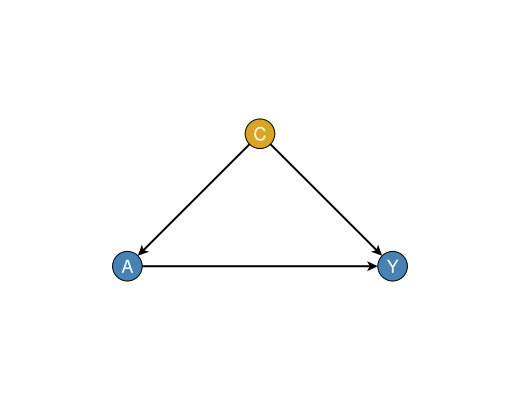
We ground the grids in a tiny SCM, treatment \(A\), outcome \(Y\), confounder \(C\):

\[ C \rightarrow A, \qquad C \rightarrow Y, \qquad A \rightarrow Y \]

Structural stratum. The graph and mechanisms:

\[ \begin{aligned} C &\coloneqq U^c \\ A &\coloneqq \mathbf{1}\{\gamma C + U^a > 0\} \\ Y &\coloneqq \beta_A A + \beta_C C + U^y \end{aligned} \]

with \(U^c, U^a, U^y\) independent standard normals. The edge \(A \rightarrow Y\) is the causal dyad of interest; \(C\) opens a backdoor \(A \leftarrow C \rightarrow Y\).

Dynamical stratum. Here “dynamics” is a single evaluation of the assignments (no time index yet; that arrives in later chapters).

Observable stratum. We observe \((A,Y)\) (and, when stated, \(C\)); \(U\) remains latent creative advance.

3.6.1 Visualising the society

Precompiling packages...
   5943.8 ms  ✓ DAGMakie
  1 dependency successfully precompiled in 7 seconds. 275 already precompiled.

Figure 3.1: Tiny confounded SCM: the causal dyad \(A \rightarrow Y\) with backdoor \(A \leftarrow C \rightarrow Y\). Dashed thinking: \(C\) is often only partially observed; here we treat it as known when adjusting.

3.6.2 Computing the three levels

include(joinpath(dirname(Base.active_project()), "scripts", "ensure_packages.jl"))
@auto_using Random Statistics

# Structural / dynamical parameters (society)
β_A = 1.0    # causal effect of A on Y
β_C = 2.0    # confounding path C → Y
γ = 1.5      # C → A

"""
    draw_exogenous(rng) -> NamedTuple

Draw one unit's creative advance `(Uᶜ, Uᵃ, Uʸ)`.
"""
function draw_exogenous(rng)
    (Uᶜ = randn(rng), Uᵃ = randn(rng), Uʸ = randn(rng))
end

"""
    simulate_unit(u; a_do=nothing) -> NamedTuple

Evaluate structural assignments for one unit.
If `a_do` is set, replace the mechanism for `A` by `do(A = a_do)`.
"""
function simulate_unit(u; a_do::Union{Nothing,Int} = nothing)
    C = u.Uᶜ
    A = a_do === nothing ? Int(γ * C + u.Uᵃ > 0) : a_do
    Y = β_A * A + β_C * C + u.Uʸ
    return (C = C, A = A, Y = Y, u = u)
end

n = 20_000
rng = MersenneTwister(2026)

# Factual population (observational regime)
units = [simulate_unit(draw_exogenous(rng)) for _ in 1:n]

# L1: association — E[Y | A = a] from observations alone
μ_L1 = (a0 = mean(x.Y for x in units if x.A == 0),
         a1 = mean(x.Y for x in units if x.A == 1))

# L2: intervention — E[Y | do(A = a)]
μ_L2 = (a0 = mean(simulate_unit(draw_exogenous(rng); a_do = 0).Y for _ in 1:n),
         a1 = mean(simulate_unit(draw_exogenous(rng); a_do = 1).Y for _ in 1:n))

# L3: counterfactual for one organism — fix u, alternative concrescence
u_star = draw_exogenous(MersenneTwister(7))
factual = simulate_unit(u_star)                         # whatever A nature assigned
cf_flip = simulate_unit(u_star; a_do = 1 - factual.A)   # same u, flipped A

assoc_contrast = μ_L1.a1 - μ_L1.a0
interv_contrast = μ_L2.a1 - μ_L2.a0
true_effect = β_A  # from the structural assignment for Y

println("L1 associative contrast E[Y|A=1]-E[Y|A=0] ≈ ", round(assoc_contrast; digits = 3))
println("L2 interventional contrast E[Y|do(A=1)]-E[Y|do(A=0)] ≈ ", round(interv_contrast; digits = 3))
println("True structural effect β_A = ", true_effect)
println("L3 unit: factual A=$(factual.A), Y=$(round(factual.Y; digits=3)); ",
        "counterfactual do(A=$(cf_flip.A)), Y=$(round(cf_flip.Y; digits=3))")

L1 associative contrast E[Y|A=1]-E[Y|A=0] ≈ 3.627
L2 interventional contrast E[Y|do(A=1)]-E[Y|do(A=0)] ≈ 1.025
True structural effect β_A = 1.0
L3 unit: factual A=1, Y=4.15; counterfactual do(A=0), Y=3.15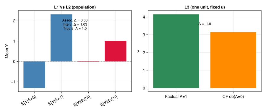

Figure 3.2: Three levels on the confounded dyad. Left: observational means \(E[Y \mid A]\) (L1) versus interventional means \(E[Y \mid do(A)]\) (L2)—confounding inflates the associative contrast. Right: one unit’s factual \(Y\) and counterfactual \(Y^{do(1-A)}(\mathbf{u})\) under shared creative advance (L3).

L1 (Seeing). From \((A,Y)\) alone we estimate \(E[Y \mid A=1] - E[Y \mid A=0]\). Because \(C\) drives both treatment and outcome, this associative contrast is larger than the causal effect \(\beta_A\).

L2 (Doing). Under \(do(A=a)\) we replace the assignment for \(A\), leaving \(C \coloneqq U^c\) and \(Y \coloneqq \beta_A A + \beta_C C + U^y\) unchanged. The interventional contrast recovers \(\beta_A\) (Monte Carlo noise aside), graph surgery answers the policy question association cannot.

L3 (Imagining). For one organism we fix the realised creative advance \(\mathbf{u}\) and replay with flipped \(A\). The factual and counterfactual \(Y\) are alternative concrescences of the same unit (Pearl 2009).

3.6.3 Summary

1. Process-over-substance: model systems as becoming, organised by strata and levels.
2. Strata locate assumptions; levels locate queries.
3. On a confounded dyad, \(E[Y \mid A] \neq E[Y \mid do(A)]\), L1 is not L2.
4. Counterfactuals require fixed \(\mathbf{u}\); they are the strongest claims and need the strongest assumptions.
5. Later chapters lift this one-step SCM into time, networks, and partial observation.

3.7 Further Reading

• Pearl (2009): Causality: foundational treatment of the hierarchy
• Bareinboim and Pearl (2016): causal inference and data fusion
• Bareinboim (2026): Causal AI (hierarchy and modern framing)
• Whitehead (1978): Process and Reality: process orientation (terms glossed in the Introduction)
• Robins (1986); Robins et al. (2000); Hernán and Robins (2020): longitudinal confounding and interventions
• Durbin and Koopman (2012); Särkkä (2013): state-space / latent dynamics

3.8 References

Bareinboim, Elias. 2026. Causal AI.

Bareinboim, Elias, and Judea Pearl. 2016. “Causal Inference and the Data-Fusion Problem.” Proceedings of the National Academy of Sciences 113 (27): 7345–52.

Durbin, James, and Siem Jan Koopman. 2012. Time Series Analysis by State Space Methods. 2nd ed. Oxford University Press.

Hernán, Miguel A., and James M. Robins. 2020. Causal Inference: What If. Chapman & Hall/CRC.

Pearl, Judea. 2009. Causality: Models, Reasoning, and Inference. 2nd ed. Cambridge University Press.

Robins, James M. 1986. “A New Approach to Causal Inference in Mortality Studies with a Sustained Exposure Period—Application to Control of the Healthy Worker Survivor Effect.” Mathematical Modelling 7 (9–12): 1393–512.

Robins, James M., Miguel A. Hernán, and Babette Brumback. 2000. “Marginal Structural Models and Causal Inference in Epidemiology.” Epidemiology 11 (5): 550–60.

Särkkä, Simo. 2013. Bayesian Filtering and Smoothing. Cambridge University Press.

Whitehead, Alfred North. 1978. Process and Reality: An Essay in Cosmology. Edited by David Ray Griffin and Donald W. Sherburne. Free Press.